Energy-Efficiency in Heterogeneous Wireless Sensor Networks
Introduction.
The use of wireless sensor networks (WSN) [1-4] has increased in the last years. They allow quick and easy data access without distance or location limits, and with low installation and maintenance costs. There are many examples of their use, in military (rescue operations, surveillance) and civilian applications (industrial control, agriculture).
An important aspect in the use of WSNs is the energy efficiency. Usually, wireless sensors are powered by batteries, and their lifetimes will be affected depending on the data transmission rates and scope, among other factors. The problem of the design of energy-efficient WSNs has been established as an NP-hard [5] problem by some authors [6, 7]. This problem has been tackled using several methodologies and criteria (objectives). For example, Konstantinids et al [8] proposed a new multi-objective evolutionary algorithm (MOEA) to optimize the coverage and power consumption, and He et al [9] used a heuristic to optimize lifetime and reliability coverage.
Nowadays, the use of heterogeneous WSNs [10, 11] including auxiliary devices (routers) to minimize the data communication, allows increasing their speed and lifetime. We can find some references about this topic. Thus, Cardei et al [12] studied the sensor position on a pre-established network to optimize coverage and energetic cost and Duarte-Melo et al. [13] the lifetime and energy consumption optimization.
Main goal.
We propose to solve the heterogeneous WSN design problem optimizing several objectives simultaneously. We do not forget that a good solution for heterogeneous WSN involves an increase of the energy efficiency compared with its homogeneous equivalent. As we have said previously, this is an NP-hard problem, so we need to use certain techniques to make easier its resolution, like the evolutionary algorithms (EAs) that are used for this purpose widely [14]. We propose to use for this problem two well-known multi-objective EAs: NSGA-II (Non-dominated Sorting Genetic Algorithm II) [15] and SPEA-II (Strength Pareto Evolutionary Algorithm II) [16].
Proposed method.
This problem tries to solve the deployment of a heterogeneous WSN like the one shown in Fig. 1. This network has several elements: a collector node (C) responsible to collect all the generated data on the network; N routers that allow to establish communications between routers and collector and collect obtained data by sensors; and M terminal nodes or sensors that obtain information about its environment. In addition, there are other important parameters that allow us to define a data instance: width (Dx) and height (Dy) of the scenery, range radius (Rr) of a router (it is the capacity of a router to establish communications with other routers and the collector node), and sensor sensitivity radius (Rs) (it is the terrain portion over which the sensor can obtain information). The definition of this problem is similar to [12].
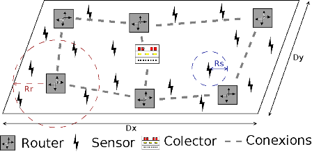
Figure 1. Deployment of a heterogeneous WSN
We propose to consider the most important factors to deploy the network. On the one hand, those that define the router network quality: average number of hops (to minimize) and reliability (to maximize); and on the other hand, the global coverage provided by sensors (to maximize). These objectives are simultaneously optimized using the MOEAs. As secondary objective, we define the number of routers. This value will be modified along several executions for the same scenery.
Some fitness functions are necessary in order to quantifying the goodness of a solution:
- Average number of hops (1): minimum number of hops between each router and collector node, divided by the total number of routers. A hop is possible when the distance between two elements is less than a fixed maximum (Rr). In (1) MinimumJumps is a function which provides the minimum number of hops between two nodes, using for this task the Dijsktra’s formulation [17].
- Sensor coverage (2): terrain percentage covered by the sensor nodes. We can found two options in the bibliography [18]. The first one focus on provided coverage by a sensor; it can be considered as a circumference of radius Rs, so the global coverage will be the intersection of all of them. The second one consists of the use of a boolean matrix over terrain, so for each sensor, the points within its radius will be activated; finally, we have to count the activated points. We have selected the second option, because although the first option is more exact, it is harder. In (2), R represents the previously boolean matrix and Rx,y the position (x,y) of this matrix.
- Reliability (3): measure that allows defining the network robustness. We have defined it as the number of the possible paths between each router and the collector node, divided by the maximum number of paths in a fully coupled topology. In (3), the function TotalRoutes provides the possible number of paths between two routers. Notice that when we use N+1 is because we have included the collector node.
Experimental datasets.
The instance data are based on a well-proven set of WSN data used in [8]. The instance represents a terrain of 100x100 meters, and a variable number of sensors and routers.
With these instances, we propose to adjust the most usual parameters for getting the suitable configurations, always based on 30 independent runs (number of evaluations, population size and crossover and mutation probabilities). Detailed information about these datasets and download site, click here.
To stabilize the goodness of solutions (Pareto fronts [14]), we propose to use the hypervolume metric [20], fixing as reference points the next ones: nadir (0.0, 10, 0.0) and ideal (1.0, 0.0, 1.0) for sensor coverage, number of hops and reliability. The reference values for coverage and reliability are simple, since they always are in a scale between 0 and 1 (probability); the number of hops implies an added complexity, so it has been necessary to fix a maximum number of hops; in this case we have considered that a value 10 is enough. Also, we recommend to perform a statistic analysis for each ideal configuration in order to determine if one of them gives significantly better results. For this task, the first step is to make a normal analysis using Shapiro-Wilk [22] and Kolmogorov-Smirnov-Lilliefors [23] tests, for determining if data come from a normal or not-normal distribution.
Current advances and developments done can be found in [25].
References.
- [1] GI. Akyildiz, W. Su, Y. Sankarasubramaniam, E. Cayirci, “A survey on sensor networks”, IEEE Communications Magazine (2002) 102–114.
- [2] Vieira, M.A.M, Coelho, C.N, Jr. da Silva, D.C. “Survey on wireless sensor network devices”. Emerging Technologies and Factory Automation, 2003. Proceedings. ETFA'03 conference.
- [3] Pottie GJ, Kaiser WJ (2000) “Wireless integrated network sensors”. Commun ACM 43(5):51–58.
- [4] Yick J, Mukherjee B, Ghosal D (2008) “Wireless sensor network survey”. Comput Netw 52(12): 2292– 2330.
- [5] M. R. Garey and D. S. Johnson, “Computers and Intractability: A Guide to the Theory of NP-Completeness”. San Francisco, CA: Freeman, 1979.
- [6] X. Cheng, B. Narahari, R. Simha, M. Cheng, D. Liu, “Strong minimum energy topology in wireless sensor networks: Np-completeness and heuristics”, IEEE Transactions on Mobile Computing 2 (3) (2003) 248–256.
- [7] A.E.F. Clementi, P. Penna, R. Silvestri, “Hardness results for the power range assignmet problem in packet radio networks”, in: Proceedings of the International Workshop on Approximation Algorithms for Combinatorial Optimization Problems, Springer-Verlag, 1999, pp. 197–208.
- [8] A. Konstantinidis y K. Yang, “Multi-objective energy-efficient dense deployment in Wireless Sensor Networks using a hybrid problem-specific MOEA/D”, Applied Soft Computing, vol. 11, págs. 4117-4134, Sep. 2011.
- [9] J. He, N. Xiong, Y. Xiao, y Y. Pan, “A Reliable Energy Efficient Algorithm for Target Coverage in Wireless Sensor Networks”, 2010, págs. 180-188.
- [10] Heterogeneous Networks with Intel XScale, http://www.intel.com/research/exploratory/heterogeneous.htm
- [11] M. Yarvis et al., “Exploiting Heterogeneity in Sensor Networks”, IEEE INFOCOM, 2005.
- [12] M. Cardei, M. O. Pervaiz, y I. Cardei, “Energy-Efficient Range Assignment in Heterogeneous Wireless Sensor Networks”, 2006, págs. 11-11.
- [13] E. J. Duarte-Melo y Mingyan Liu, “Analysis of energy consumption and lifetime of heterogeneous wireless sensor networks”, vol. 1, págs. 21-25.
- [14] K. Deb, “Multiobjective optimization using evolutionary algorithms”. New York;;Chichester: Wiley, 2001.
- [15] Kalyanmoy Deb, Samir Agrawal, Amrit Pratap and T Meyarivan, “A Fast Elitist Non-dominated Sorting Genetic Algorithm for Multi-objective Optimization: NSGA-II”, Parallel Problem Solving from Nature PPSN VI, 2000.
- [16] E. Zitzler, M. Laumanns and L. Thiele, “SPEA2: Improving the strength Pareto evolutionary algorithm”, EUROGEN 2001.
- [17] T. Cormen, “Introduction to algorithms”, Cambridge Mass.: The MIT Press, 2001
- [18] M. Younis y K. Akkaya, “Strategies and techniques for node placement in wireless sensor networks: A survey”, Ad Hoc Networks, vol. 6, págs. 621-655, Jun. 2008.
- [19] "A Multi-Objective Network Design for Real Traffic Models of the Internet by means of a Parallel Framework for Solving NP-Hard Problems". José M. Lanza-Gutiérrez, Juan A. Gómez-Pulido, Miguel A. Vega-Rodríguez, Juan M. Sánchez-Pérez. Proceedings of the Third World Congress on Nature and Biologically Inspired Computing, IEEE Computer Society, Salamanca, Spain, 2011, pag:144-149. ISBN:978-1-4577-1123-7.
- [20] Fonseca, C., Knowles, J., Thiele, L., Zitzler, E. , “A Tutorial on the Performance Assessment of Stochastic Multiobjective Optimizers”, EMO 2005.
- [21] José Otero, Luciano Sánchez, “Diseños Experimentales y Tests Estadísticos”, Tendencias Actuales en Machine Learning V Congreso Español sobre Metaheurísticas, Algoritmos Evolutivos y Bioinspirados, MAEB 07 Tenerife, Spain 2007
- [22] Shapiro, S. S. and Wilk, M. B, “An analysis of variance test for normality”, Biometrika, 52, 3 and 4, (1965) 591-611
- [23] Chakravarti, Laha, and Roy, “Handbook of Methods of Applied Statistics”, Volume I, John Wiley and Sons, (1967). 392-394.
- [24] Wilcoxon, F. “Individual Comparisons by Ranking Methods”. Bio-metrics 1, (1945) 80-83.
- [25] "MultiObjective Evolutionary Algorithms for Energy-Efficiency in Heterogeneous Wireless Sensor Networks". José M. Lanza-Gutiérrez, Juan A. Gómez-Pulido, Miguel A. Vega-Rodríguez, Juan M. Sánchez-Pérez. Proceedings of the 2012 IEEE Sensors Applications Symposium (SAS 2012), IEEE, Brescia, Italy, 2012, pag:194-199. ISBN:978-1-4577-1723-9.
Coordinator/contact:
- Esta dirección electrónica esta protegida contra spam bots. Necesita activar JavaScript para visualizarla .
- Esta dirección electrónica esta protegida contra spam bots. Necesita activar JavaScript para visualizarla .